Simulating the value of replacements for scouting football players
July 27, 2020
Role, Ability, and Value
Role
In order to quantify how one player will perform in the role of another, first we need to quantify what that role actually is. Player roles can be both well-defined or loosely-defined in football - we can say for sure that Trent Alexander-Arnold and Kyle Walker are both right-backs, but can we answer for do we describe Walker as an "inverted full-back", as Manchester City are claimed to use, and is TAA really that similar to a "traditional" right back when he plays in Liverpool's system, which pushes their full-backs way out wide when attacking. How can we define these roles based on event data from games?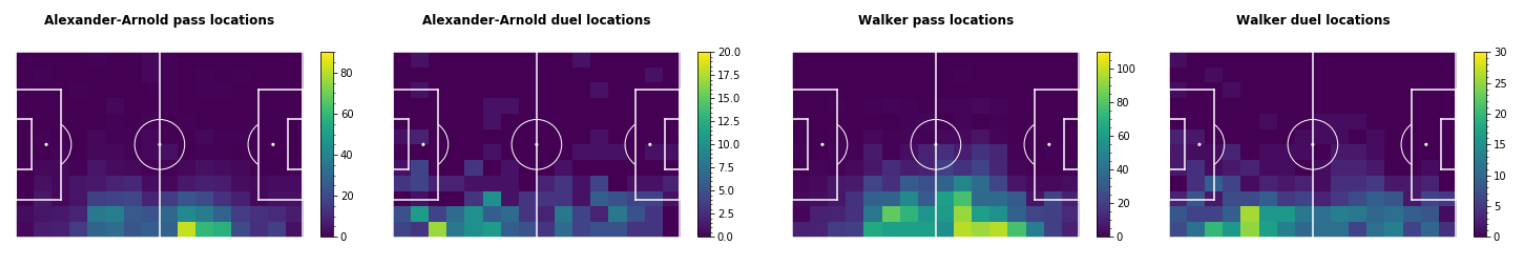


This definition isn't very exciting or seemingly clearly defined at all, but it will make more sense once we start talking about Value and see how it fits in.
Ability
When we talk about replacing one player with another, we're talking about replacing their playing ability with another player's ability. Replacing a League One striker with Messi, you're getting a player who's more able at scoring, dribbling, and creating chances. So what do we mean by ability? I'll choose to define this as the probability that a player will complete particular actions on a football pitch. If we think of the success of footballing actions as being binomial variables, player ability corresponds to the probabilities assigned to those actions. This is pretty straightforward - a really good player is able to do lots of things - complete different types of passes, score from shots, make tackles, etc. - with a high success rate.
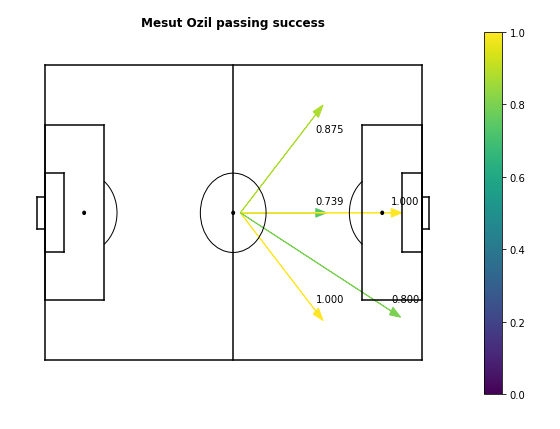
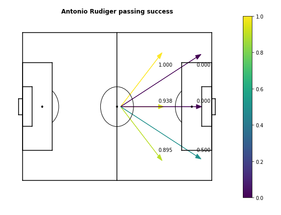
For example, we know that Mesut Ozil is an extremely good passer, specializing in defense-splitting passes in the final third. By this definition of player ability, Mesut Ozil is a good passer because he has a high probability of completing these types of passes. To illustrate, here's a passing map for Ozil, counting passes starting from the central midfield area. Let's compare him to someone who's an ok-ish passer, like Chelsea defender Antonio Rudiger.
Value
Now we need a method of quantifying how much value a player adds in a role. This requires using player ability in the context of player role - a player who's very good at long shots doesn't add much value if they aren't taking very many. For this I use the xT/VAEP framework of "valuing on-the-ball actions". You can read more about both ideas in the linked post, in the original blog post on xT, or in the original paper on VAEP This framework assigns a certain value \( V(S_i) \) to each game state \( S_i \), based on how valuable that state is. For \( xT \), which focuses on offense, \( V(S_i) \) models the probability that the team will soon score a goal. VAEP extends this to defense and models \( V_{score}(S_i) - V_{concede}(S_i) \), incorporating the probability of conceding a goal. For this piece I'll be using \( xT \), and I'll only be focusing on offensive value. \( xT \) splits a football field into \( L \times W \) total cells, and assigns a value \( V(S_i) \) to each cell, representing the probability of a goal happening if the team has possession in that cell. \( xT \) is different from \( xG \) (expected goals) and \( xA \) (expected assists) - \( xT \) represents the probability of a goal happening in any future point of that possession. The above \( xT \) visualization for Liverpool's 2017-18 team illustrates this, as opposition byline areas have relatively high \( xT \) due to a high chance of a cross leading to a goal - while in contrast those areas typically have low \( xG \) due to the low chance of scoring from a tight angle. Now for the math (which will be required later on), all that \( xT \) requires is some conditional probability and recursive relations. The equation for \( xT \) is as follows: $$ xT_{x,y} = (s_{x,y} \times g_{x,y}) + (m_{x,y} \times \sum_{z=1}^L \sum_{w=1}^W T_{(x,y) \rightarrow (z,w)} xT_{z,w}) $$ where:
\( xT_{x,y} \) is the \( xT \) in cell \( x,y \)
\( s_{x,y} \) is the probability of a shot
\( m_{x,y} \) is the probability of a pass/move
\( g_{x,y} \) is the probability of scoring from position \( x,y \) (i.e. \( xG \))
\( T_{(x,y) \rightarrow (z,w)} \) is the probability of completing a pass from cell \( x,y \) to cell \( z,w \), and
\( xT_{z,w} \) is the \( xT \) in cell \( z,w \).
Since this definition is recursive, \( xT \) is approximately solved with dynamic programming, by computing
the
probability
of scoring within the next \( K \) actions. Typically an \( xT \) model for will converge within 30-60
iterations
(\(
K \) ~ 30-60).
\( xT \) gives us a model for valuing game states (i.e. positions on a pitch), but we still need to quantify
the value \( U \) that a player adds to a team. Using the \( xT \) framework, value can be added in 2 ways: by
moving the ball (pass, cross, dribble)
and by taking a shot.
\( s_{x,y} \) is the probability of a shot
\( m_{x,y} \) is the probability of a pass/move
\( g_{x,y} \) is the probability of scoring from position \( x,y \) (i.e. \( xG \))
\( T_{(x,y) \rightarrow (z,w)} \) is the probability of completing a pass from cell \( x,y \) to cell \( z,w \), and
\( xT_{z,w} \) is the \( xT \) in cell \( z,w \).
- By moving the ball: \( U = V(S_j) - V(S_i) \) By successfully moving the ball, a player changes the state of the game from \( S_i \) to \( S_j \), thus adding value \( V(S_j) - V(S_i) \) to the team.
- By taking a shot: \( U = xG(S_i) - V(S_i) \) While in possession of the ball in state \( S_i \), there is \( V(S_i) \) chance of the possession ending in a goal. By taking a shot, there is now \( xG(S_i) \) chance of the possession (which ends in a shot) ending in a goal, thus adding \( xG(S_i) - V(S_i) \) value.
- Value added by player actions can also be negative - players can make poor passing decisions which lower the chance of scoring, or they can take bad shots when better passing options were available
- The \( xG \) model used for shot value can be team-specific or player-specific - in this piece I opt to use very basic, location-based, player-specific \( xG \) models.
Putting it all together
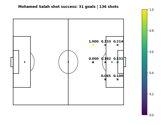
Now that we have our definitions of Role, Ability, and Value, we can put them together to simulate how players will perform in certain roles. Let's start this way: We have player \( P1 \), who plays for team \( T1 \), and player \( P2 \), who we're considering as a replacement for \( P1 \). Over the course of a season, or a match, \( P1 \) performs some actions for \( T1 \), each action adding a certain value for the team, and each action being a success or failure. For the sake of this example, let's say \( P1 \) is Mohamed Salah, \( T1 \) is Liverpool's 2017-18 team, and \( P2 \) is Mesut Ozil. Let's take a look at some of Salah's actions during Liverpool's 4-3 win over Man City in January 2018.
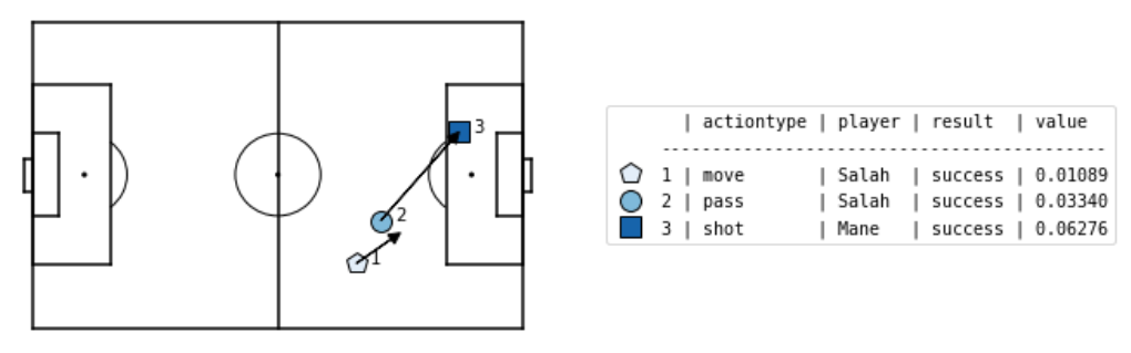

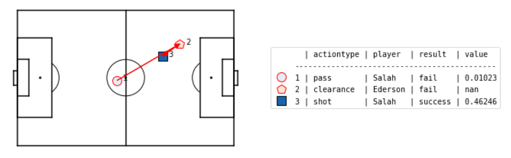
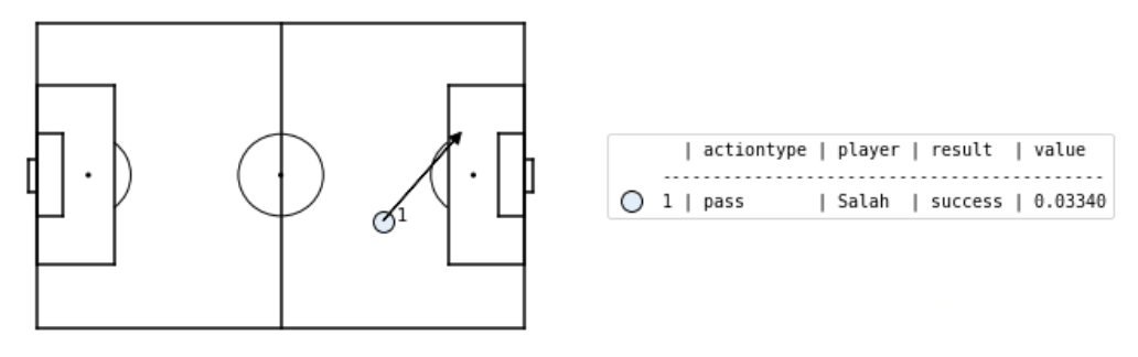
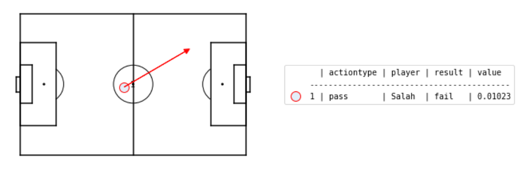
If you haven't guessed by now, I'm a Liverpool fan. In the first sequence leading up to Sadio Mane's goal, Salah produces a pass (action #2) to Mane, from about 30 metres out on the right, to the left edge of the box. This pass succeeds, and according to our \( xT \) model has value 0.0334. In the second sequence, Salah attempts another pass to Mane (action #1), but the pass is intercepted by Ederson. This would have had value 0.0102, but was not a success. Looking at just the 2 passes alone, we can say the indicator variable of success for the 1st pass was \( 1 \), while the indicator variable of success for the 2nd pass was \( 0 \).
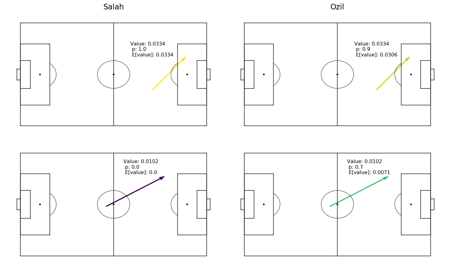
Just a tiny bit more (recomputing the \( xT \) model)
But wait, there's something not right yet - if we're replacing Salah with Ozil, we can't compute value added based on the old \( xT \) model. Suppose we change our scenario, and we're replacing some very average League One striker who plays for a League One team, with Lionel Messi. Since Messi likely has a higher pass and shot success probability, the \( xT \) model that includes Messi should automatically value its game states more. Thinking about a single action, the value of a successful forward pass should now change, because there's now a higher probability of a goal since Messi could end up on the end of that pass. Revisiting the original \( xT \) equation, what we have to modify is \( g_{x,y} \) and \( T_{(x,y) \rightarrow (z,w) } \), while keeping \( s_{x,y} \) and \( m_{x,y} \) the same. What this means is we're keeping the actions made the same - we assume replacing a player has no influence on playing style - but modifying the probability that the actions will be successful. For \( g_{x,y} \) the modification is quite simple: $$ g_{x,y}' = N^{P1} g_{x,y}^{P2} + \frac{N - N^{P1}}{N} g_{x,y}^{T1 - P1} $$ where:
\( N \) is the number of shots taken by team \( T1 \) from location \( x,y \)
\( N^{P1} \) is the number of shots taken by player \( P1 \) from location \( x,y \)
\( g_{x,y}^{P2} \) is the shot accuracy of player \( P2 \) from location \( x,y \) and
\( g_{x,y}^{T1 - P1} \) is the shot accuracy of the players in team \( T1 \), excluding \( P1 \), from location \( x,y \)
For \( T_{(x,y) \rightarrow (z,w)} \) this becomes a bit trickier:
$$
T_{(x,y) \rightarrow (z,w)}' = p_{(x,y) \rightarrow (z,w)} \times [ N^{P1} T_{(x,y) \rightarrow (z,w)}^{P2} +
\frac{N - N^{P1}}{N} T_{(x,y) \rightarrow (z,w)}^{T1-P1} ]
$$
where:
\( N^{P1} \) is the number of shots taken by player \( P1 \) from location \( x,y \)
\( g_{x,y}^{P2} \) is the shot accuracy of player \( P2 \) from location \( x,y \) and
\( g_{x,y}^{T1 - P1} \) is the shot accuracy of the players in team \( T1 \), excluding \( P1 \), from location \( x,y \)
\( N \) is the number of passes attempted by team \( T1 \) from location \( x,y \) to location \( z,w \)
\( N^{P1} \) is the number of passes attempted by player \( P1 \) from location \( x,y \) to location \( z,w \)
\( p_{(x,y) \rightarrow (z,w)} \) is the probability of team \( T1 \) choosing to pass to location \( z,w \) given that they choose to pass from location \( x,y \)
\( T_{(x,y) \rightarrow (z,w)}^{P2} \) is the probability that player \( P2 \) completes a pass from location \( x,y \) to location \( z,w \)
\( T_{(x,y) \rightarrow (z,w)}^{T1-P1} \) is the probability that team \( T1 \), excluding player \( P1 \), completes a pass from location \( x,y \) to location \( z,w \)
Essentially we're measuring the pass & shot accuracy, if we had \( P2 \) take all the passes and shots that \(
P1 \) did for team \( T1 \).
\( N^{P1} \) is the number of passes attempted by player \( P1 \) from location \( x,y \) to location \( z,w \)
\( p_{(x,y) \rightarrow (z,w)} \) is the probability of team \( T1 \) choosing to pass to location \( z,w \) given that they choose to pass from location \( x,y \)
\( T_{(x,y) \rightarrow (z,w)}^{P2} \) is the probability that player \( P2 \) completes a pass from location \( x,y \) to location \( z,w \)
\( T_{(x,y) \rightarrow (z,w)}^{T1-P1} \) is the probability that team \( T1 \), excluding player \( P1 \), completes a pass from location \( x,y \) to location \( z,w \)
The sparsity issue (can skip this section)
There's still a couple of issues with this method, and you might have noticed some of them already. One that I'll address is an issue of sparsity for event locations. Since the move & shot probability models are based on limited data, move & shot probability cells will be non-zero only if the player has completed an action in that cell. Many values of \( g_{x,y}^{P2} \) and \( T_{(x,y) \rightarrow (z,w)}^{P2} \) will be \( 0 \). Another issue is unrealistic probability values due to small sample data. For example, Mohamed Salah's long range goal against Man City was the only shot Salah took from that area all season. That gives him a shot probability of \( 1.0 \) from that cell, which is extremely unrealistic. The same principle applies for passes - this skews the ability of players when we're simulating them. In short, there's 2 main problems:- Some cells may have low or zero probability when they're actually good goal-scoring/passing locations.
- Some cells may have high probability when they're bad goal-scoring/passing locations, due to small samples.
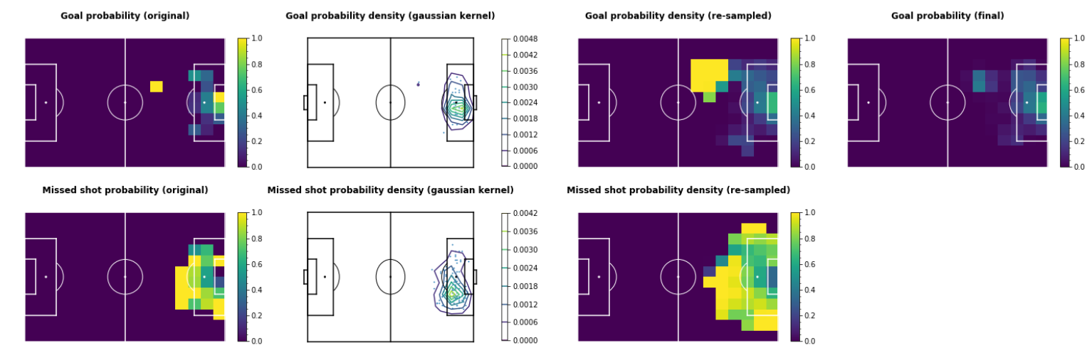
- Separate all shot events into goals & missed shots (successful/unsuccessful moves for move events), creating an array of 2D coordinates for each (shapes of \( N_g \times 2 \) and \( N_m \times 2 \)).
- For both goals & missed shots, perform Kernel Density Estimation with a Gaussian kernel. For this a kernel bandwidth of \( 2.5 \) is used.
- Resample \( N_g \) goal locations and \( N_m \) missed shot locations from the estimated densities, repeat this for \( 1000 \) iterations and compute the average. This "expands" the set of event locations, and increases the probability for cells with neighboring high-probability cells.
-
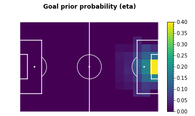
Use a prior \( xG \) grid, \( \eta \) to smooth both matrices. For this work, this grid is constructed
from
all available shot events from the 2017-18 season.
The number of shots & goals are counted per grid cell, and any cell with \( < 5 \) goals is set to \( 0 \)
to avoid outliers, before dividing by the number of shots.
The resulting grid \( \eta \) is then used in the following manner: Where \( G_{x,y} \) and \( M_{x,y} \) are the goal & missed shot counts, and \( \alpha \) is a parameter controlling the amount of smoothing - for this piece I use \( alpha = 0.6 \). - Finally, return the resulting matrix \( g \), where: $$ g_{x,y} = \frac{G_{x,y}}{G_{x,y} + M_{x,y}} $$
Seeing it in action
FINALLY. Now that we know how to do this, let's see the actual results. Let's try finding a replacement for 2017-18 Mohamed Salah. To do this, we'll take all the players in Europe's top 5 leagues who scored at least 10 league goals in 2017/18, and simulate them in place of Salah. Let's take a look at the top 10 players, sorted by expected value added.
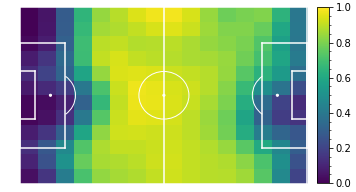
Pass accuracy per position
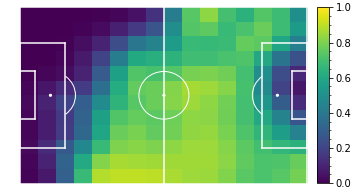
Shot accuracy per position
Shot accuracy per position

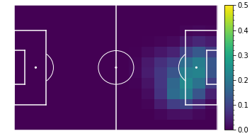
Mohamed Salah (Liverpool)
Move value: 5.968
Shot value: 13.656
Total value: 19.624
Move value: 5.968
Shot value: 13.656
Total value: 19.624
Pass accuracy per position
Shot accuracy per position
Shot accuracy per position

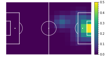
Paulo Dybala (Juventus)
Move value: 5.710
Shot value: 21.545
Total value: 27.255
Move value: 5.710
Shot value: 21.545
Total value: 27.255
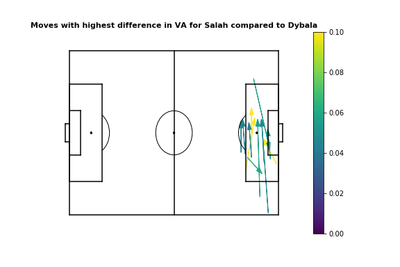
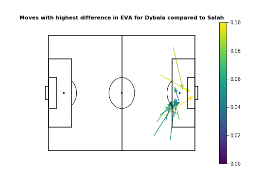
From visualizing the top 12 moves for each player, we see that Dybala provides more value when moving the ball into the box from the right, or when penetrating from the center/left. On the other hand, Salah adds more value with passes across the penalty area, either when crossing or moving the ball to Firmino/Mane.
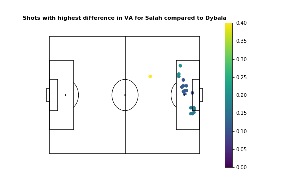
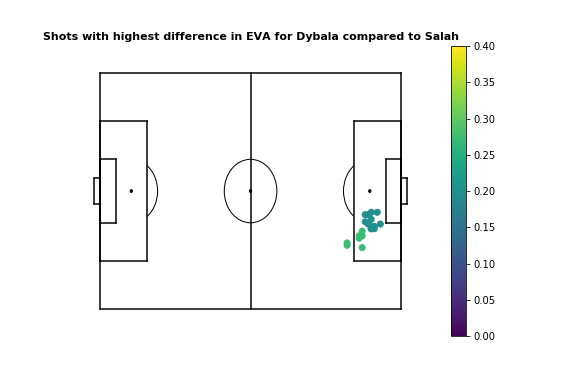
With shots this becomes a bit more difficult to interpret. The concept of value added per shot is a bit strange - shots with a high \( xG \) may actually subtract value in areas with high \( xT \). However, the comparative plots are still intuitive, as following their shooting accuracy plots, Salah adds more value than Dybala when shooting from the center, left, or the right edge of the 6-yard box, while Dybala adds more value when shooting from the right edge of the box. You can try seeing the results for different players by yourself. Here's the evaluation for the top 100 value creators in Europe's top 5 leagues during the 2017-18 season.
Team
Player
Limitations & future work
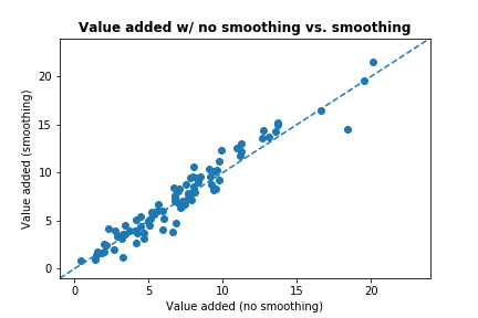
Obviously there are several limitations to this work, and several ways in which it can be improved on. Some of these limitations are in terms of the technical methods used and scope of the work, and some are due to the limited nature of the available data. Some areas for improvement which would be interesting are:- Extension to defensive value/VAEP framework: The current framework only uses the \( xT \) model of value creation, which only considers offensive value added by players. An initial extension to include defensive contribution while still using the \( xT \) model would be relatively straightforward and interesting. Another limitation of the \( xT \) framework is that the value per action is only a function of location, and an extension of this to the VAEP framework which relies more on predictive modeling would be very useful. However, one issue where the solution isn't immediately obvious is how an VAEP model should be updated following the inclusion of a player (in the same manner as the \( xT \) modification section above). With \( xT \) the value model is constructed from the success probability matrices so updating the probabilities is sufficient, but I'm not sure how this would be done with a predictive model.
- Evaluation for team-level changes in expected value added: The current method only evaluates the change in value added for the player replaced. However, modifying one player in the \( xT \) framework leads to different action values for all players in the team - a pass to Messi leads to more threat than a pass to a League One striker - and so inclusion of team-level value would be interesting. We might end up seeing some players that add small marginal value in their own roles when simulated, but add a large amount of value to the overall team.
- Better models/data for action success probabilities: The current shot probability & move probability values are calculated based only on the locations, without taking into account the difficulty of the pass. A simple ground pass with no defenders in the way, and a lofted through ball past 3 players are valued the same in the current setup. Better player-level models that account for variables like defender positioning, defensive pressure, type of pass (air, ground, footedness, etc.) would be interesting if we could incorporate a VAEP-like framework. Furthermore, event sparsity is still an issue even with smoothing. You might have noticed that Illaramendi scores extremely high in the EVA replacement rankings - this is due to him scoring 3 goals from 3 shots in one particular penalty area grid cell.
- Better understanding of failed actions: Locations for events like failed passes and dribbles are still listed in the data as the actions occurred, not as they were intended. For example, a through ball intended into the penalty box that was intercepted at the edge of the box, is still listed as a pass to the edge of the box. Better ways for dealing with these actions would lead to a more accurate evaluation of the expected value added by them.